geobounds

[!IMPORTANT]

Attribution is required when using geoBoundaries.

Why this package?

The geobounds package provides an R-friendly interface for accessing and using the geoBoundaries dataset, a global database of administrative boundary polygons. Using this package, you can:

• Programmatically retrieve administrative boundary geometries, such as country boundaries and subnational administrative levels, from geoBoundaries.
• Use tidyverse and sf workflows in R to map, analyze and join these boundaries with your own data.
• Work in an open-data context where attribution to geoBoundaries is required.

In short, if you work with administrative boundaries in R, this package simplifies downloads, caching and integration with other spatial data.

Installation

Install geobounds from CRAN:

install.packages("geobounds")

# install.packages("pak")
pak::pak("dieghernan/geobounds")

# Install geobounds in R:
install.packages(
  "geobounds",
  repos = c(
    "https://dieghernan.r-universe.dev",
    "https://cloud.r-project.org"
  )
)

Example usage

library(geobounds)

sri_lanka_adm1 <- gb_get_adm1("Sri Lanka")
sri_lanka_adm2 <- gb_get_adm2("Sri Lanka")
sri_lanka_adm3 <- gb_get_adm3("Sri Lanka")

library(sf)
library(dplyr)

library(ggplot2)

ggplot(sri_lanka_adm3) +
  geom_sf(fill = "#DFDFDF", color = "white") +
  geom_sf(data = sri_lanka_adm2, fill = NA, color = "#F0B323") +
  geom_sf(data = sri_lanka_adm1, fill = NA, color = "black") +
  labs(caption = "Source: www.geoboundaries.org") +
  theme_void()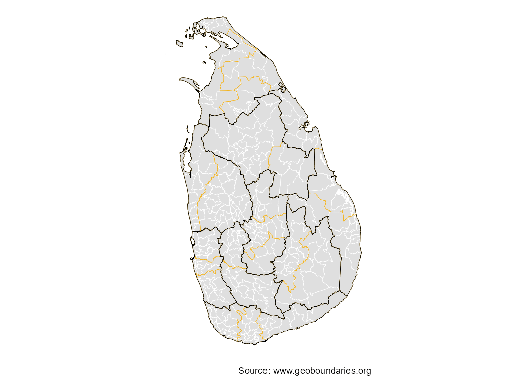

Release types

geoBoundaries offers different release types with varying sources, validation processes and licensing:

• gbOpen: Freely available boundaries under CC BY 4.0, suitable for most uses when attribution is provided.
• gbHumanitarian: Boundaries mirrored from UN OCHA for humanitarian use, which may have less open licensure.
• gbAuthoritative: Boundaries mirrored from UN SALB and verified through in-country processes, and cannot be used for commercial purposes.

Use the release_type argument in functions to specify, for example, gb_get_adm1("Sri Lanka", release_type = "gbHumanitarian").

For detailed comparisons, see the vignettes.

Advanced usage

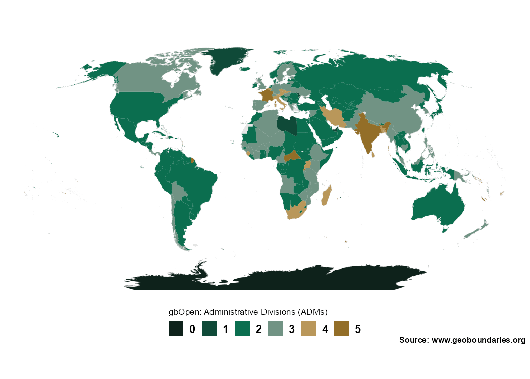
Map the highest available administrative level in geoBoundaries by country:

library(geobounds)
library(ggplot2)
library(dplyr)

world <- gb_get_world()
max_lvl <- gb_get_max_adm_lvl(release_type = "gbOpen")

world_max <- world |>
  mutate(boundaryISO = shapeGroup) |>
  left_join(max_lvl) |>
  mutate(max_lvl = factor(maxBoundaryType, levels = 0:5))

pal <- c("#0e221b", "#0f4a38", "#0b6e4f", "#719384", "#b9975a", "#936e28")
names(pal) <- levels(world_max$max_lvl)

ggplot(world_max) +
  geom_sf(fill = "#e5e5e5", color = "#e5e5e5") +
  geom_sf(aes(fill = max_lvl), color = "transparent") +
  scale_fill_manual(values = pal, na.translate = FALSE, drop = FALSE) +
  guides(fill = guide_legend(direction = "horizontal", nrow = 1)) +
  coord_sf(expand = TRUE, crs = "+proj=robin") +
  theme_void() +
  theme(
    plot.background = element_rect(fill = "white", color = NA),
    text = element_text(family = "sans", face = "bold"),
    legend.position = "bottom",
    legend.title.position = "top",
    legend.title = element_text(size = rel(0.75), face = "plain"),
    legend.text = element_text(size = rel(1)),
    legend.text.position = "right",
    legend.key.height = unit(1, "line"),
    legend.key.width = unit(1, "line"),
    plot.caption = element_text(
      size = rel(0.7),
      margin = margin(r = 4)
    )
  ) +
  labs(
    fill = "gbOpen: Administrative levels (ADMs)",
    caption = "Source: www.geoboundaries.org"
  )

Documentation and resources

• Visit the pkgdown site for full documentation: https://dieghernan.github.io/geobounds/
• Vignettes on data releases:
  • gbOpen
  • gbHumanitarian
  • gbAuthoritative
• Explore the geoBoundaries homepage: https://www.geoboundaries.org/
• Read the original paper describing the geoBoundaries dataset (Runfola et al. 2020).
• Report issues or contribute on GitHub.

License

This package is released under the CC BY 4.0 license. The default geoBoundaries release type, gbOpen, is CC BY 4.0 compliant when attribution is provided. Other release types may have additional licensing limits, so check the metadata returned by gb_get_metadata() before reuse.

Acknowledgements

• Many thanks to the geoBoundaries team and the William & Mary geoLab for creating and maintaining the dataset.
• Thanks to the R package community and all contributors to this package’s development.
• If you use geobounds and the underlying geoBoundaries data in your research or projects, please cite and acknowledge them.

Citation

Hernangómez D (2026). geobounds: Download Administrative Boundary Data from geoBoundaries. doi:10.32614/CRAN.package.geobounds. https://dieghernan.github.io/geobounds/.

A BibTeX entry for LaTeX users:

@Manual{R-geobounds,
  title = {{geobounds}: Download Administrative Boundary Data from geoBoundaries},
  author = {Diego Hernangómez},
  year = {2026},
  version = {0.1.2},
  url = {https://dieghernan.github.io/geobounds/},
  abstract = {Tools for downloading administrative boundary data from geoBoundaries <https://www.geoboundaries.org/> across multiple administrative levels. Boundary data are returned as sf objects for mapping and spatial analysis. See Runfola, D. et al. (2020) "geoBoundaries: A global database of political administrative boundaries." PLOS ONE 15(4), e0231866. <doi:10.1371/journal.pone.0231866>.},
  doi = {10.32614/CRAN.package.geobounds},
}

References